Decision Trees

Type
Classification, Regression

Decision Trees are non-parametric supervised learning methods used for classification and regression. They use a tree-like graph of decisions to predict the value of a target variable.

Decision Tree Algorithms

CART
C4.5
C5.0

Key Components

Nodes: Represent a test on an attribute (feature).
Branches: Represent the outcome of the test.
Leaves: Represent the final class label or value.

Building the Tree (Recursive Partitioning)

The goal is to partition data into subsets that are as “pure” as possible.

Information Gain: Measures the reduction in Entropy (disorder) after a split. Higher gain is better.
Gini Impurity: A measure of how often a randomly chosen element would be incorrectly labeled. Used frequently in the CART algorithm. For class proportions $p_{k}$ in a node: $G = 1 - \sum_{k} p_{k}^{2}$ . It is 0 for a pure node and maximal ( $1 - 1/ K$ ) when all $K$ classes are equally mixed.
Splitting Criteria: At each node, the algorithm selects the feature and split point that maximizes purity in the resulting child nodes.

Overfitting and Pruning

Decision trees can easily overfit by becoming too deep and capturing noise.

Pre-pruning: Stop growing the tree early (e.g., limit depth or minimum samples per leaf).
Post-pruning: Grow the full tree and then remove nodes that provide little predictive power.

Feature	Decision Trees	Boosting
Model Type	Single base learner	Ensemble of learners
Training	Fast, recursive	Sequential, slower
Complexity	Easy to interpret	High predictive power, “black box”
Variance	High (prone to overfitting)	Reduced via iterative refinement

Example: Iris Dataset

A scikit-learn DecisionTreeClassifier trained on half of the Iris data (75 flowers, stratified split so each species has 25). The tree is exported with export_graphviz and rendered with pydotplus:

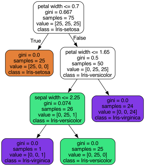
How to read a node: the top line is the test (go left if true), gini is the node’s impurity, samples is how many training flowers reach it, value is the class counts [setosa, versicolor, virginica], and class is the majority class. Color encodes the class and darker means purer.

Root: Gini = 0.667 = $1 - 3 \cdot (1/3)^{2}$ , the worst case for three balanced classes. A single test, petal width <= 0.7, isolates all 25 setosa into a pure leaf (Gini 0).
Second split: the remaining 50 flowers (Gini 0.5 = $1 - 2 \cdot (1/2)^{2}$ ) are split at petal width <= 1.65. The right branch is pure virginica (24 flowers).
Third split: the left branch has 25 versicolor and 1 virginica (Gini 0.074). One more split on sepal width <= 2.25 isolates that stray flower into its own leaf.
The final tree has only 3 splits and 4 leaves and fits the training data perfectly. Petal width does almost all the work; petal length and sepal length are never used.
The last leaf holds a single sample, a sign the tree is memorizing a training point. Compare training and test accuracy to check for overfitting, and use pruning (max_depth, min_samples_leaf, ccp_alpha) if the gap is large.

Predicting New Flowers

Predictions follow one root-to-leaf path. Three hand-made flowers (sepal length, sepal width, petal length, petal width in cm):

Example	Features	Path	Prediction
1	5.5, 3.0, 1.6, 0.2	petal width 0.2 <= 0.7	Iris-setosa
2	6.0, 2.8, 7.5, 1.4	petal width 1.4 > 0.7, <= 1.65; sepal width 2.8 > 2.25	Iris-versicolor
3	3.7, 1.1, 0.6, 2.4	petal width 2.4 > 0.7, > 1.65	Iris-virginica

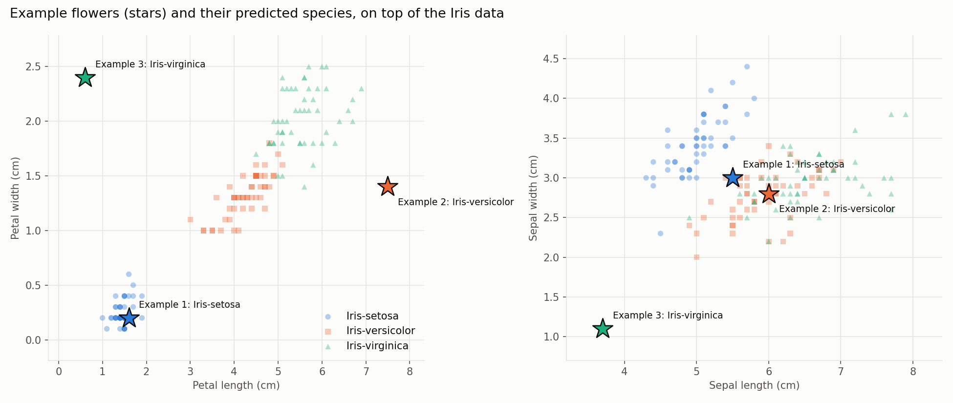
Examples 2 and 3 are deliberately unrealistic (petal length 7.5 cm with petal width 1.4 cm, or a 1.1 cm sepal width) and sit far from any real cluster. The tree still answers confidently because it only checks the features it split on: Example 2’s huge petal length is never examined, and Example 3 is called virginica purely from its petal width. Decision trees give no warning when an input lies outside the training distribution.

Code

from sklearn import tree
from sklearn.model_selection import train_test_split
 
X_train, X_test, y_train, y_test = train_test_split(
    X, y, test_size=0.5, random_state=0, stratify=y)
 
clf = tree.DecisionTreeClassifier(random_state=0).fit(X_train, y_train)
clf.predict(samples)          # class labels
clf.predict_proba(samples)    # leaf class proportions
 
dot = tree.export_graphviz(clf, feature_names=list(X.columns),
                           class_names=list(clf.classes_),
                           filled=True, rounded=True, out_file=None)

The unsupervised counterpart on the same data is k-Means; ensembles of trees are covered in Random Forest, Bagging, and Boosting.

Explorer