k-Means

Type
Clustering (unsupervised)

k-Means partitions $n$ unlabeled points into $k$ clusters, each represented by its centroid (the mean of its members). Every point belongs to the cluster whose centroid is nearest, so the result is a set of convex, roughly spherical groups. It is a non-hierarchical method, in contrast to Hierarchical Clustering.

Objective

k-Means minimizes the within-cluster sum of squares (called inertia in scikit-learn):

$J={\sum }_{j=1}^k{\sum }_{x_i\in C_j}\Vert x_i-{\mu }_j{\Vert }^2$

where ${\mu }_j$ is the centroid of cluster $C_j$. Finding the global minimum is NP-hard, so Lloyd’s algorithm is used instead and only guarantees a local minimum.

Lloyd’s Algorithm

flowchart LR
    A[Pick k initial centroids] --> B[Assign each point to nearest centroid]
    B --> C[Recompute each centroid as the mean of its points]
    C --> D{Assignments changed?}
    D -- yes --> B
    D -- no --> E[Converged]

1. Initialize $k$ centroids (random points, or the smarter k-means++ seeding that spreads them apart).
2. Assign every point to its nearest centroid (Euclidean distance).
3. Update each centroid to the mean of the points assigned to it.
4. Repeat 2-3 until assignments stop changing.

Each step can only decrease $J$, so the algorithm always converges, but the answer depends on the starting centroids. Run it several times (n_init=10 in scikit-learn) and keep the run with the lowest inertia.

Practical Notes

• Choosing $k$: the elbow method (plot inertia vs. $k$ and look for the bend) or the silhouette score (see Clustering Evaluation Metrics). Inertia always falls as $k$ grows, so it cannot be used alone.
• Scale your features: distances dominate the result, so features with large ranges overwhelm the others. See Scaling Techniques.
• Cluster labels are arbitrary: “cluster 0” in one run may be “cluster 2” in the next. Any evaluation against ground truth must be label-permutation invariant (purity, Rand index, and so on).
• Weaknesses: assumes similar-sized, spherical clusters; sensitive to outliers (means get pulled); needs $k$ upfront. Mixtures of Gaussians relaxes the shape assumption with soft assignments, and Locally Adaptive Clustering (LAC) handles clusters that live in different feature subspaces.

Example: Iris Dataset

The Iris dataset has 150 flowers (50 each of Iris-setosa, Iris-versicolor, Iris-virginica) described by four measurements: sepal length, sepal width, petal length, petal width. Running k-Means with $k=3$ on the four features, without using the species labels, and then comparing clusters to the true species:

Cluster	setosa	versicolor	virginica
0	0	48	14
1	50	0	0
2	0	2	36

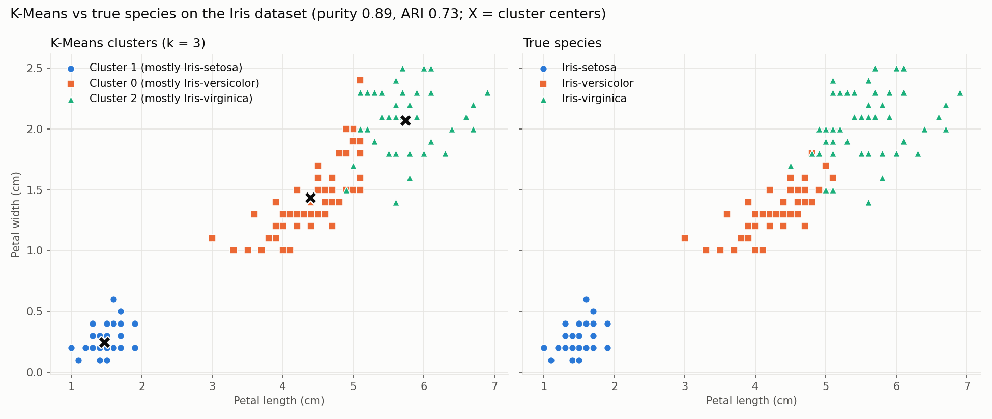
• Cluster 1 is exactly setosa: that species is linearly separable from the others.
• Clusters 0 and 2 split versicolor and virginica with 16 flowers on the wrong side, because those two species overlap.
• Purity = (50 + 48 + 36) / 150 = 0.89 and Adjusted Rand Index = 0.73. Both are computed in Clustering Evaluation Metrics.

Fitted centroids (cm):

Cluster	sepal length	sepal width	petal length	petal width
0 (mostly versicolor)	5.90	2.75	4.39	1.43
1 (mostly setosa)	5.01	3.43	1.46	0.25
2 (mostly virginica)	6.85	3.07	5.74	2.07

Petal features separate the groups cleanly. Clusters (left) closely match the true species (right); the black X marks are centroids:

Sepal features overlap much more, so the two plots look noticeably different where versicolor and virginica meet. Clustering used all four features, so a 2D slice can only show part of the structure:

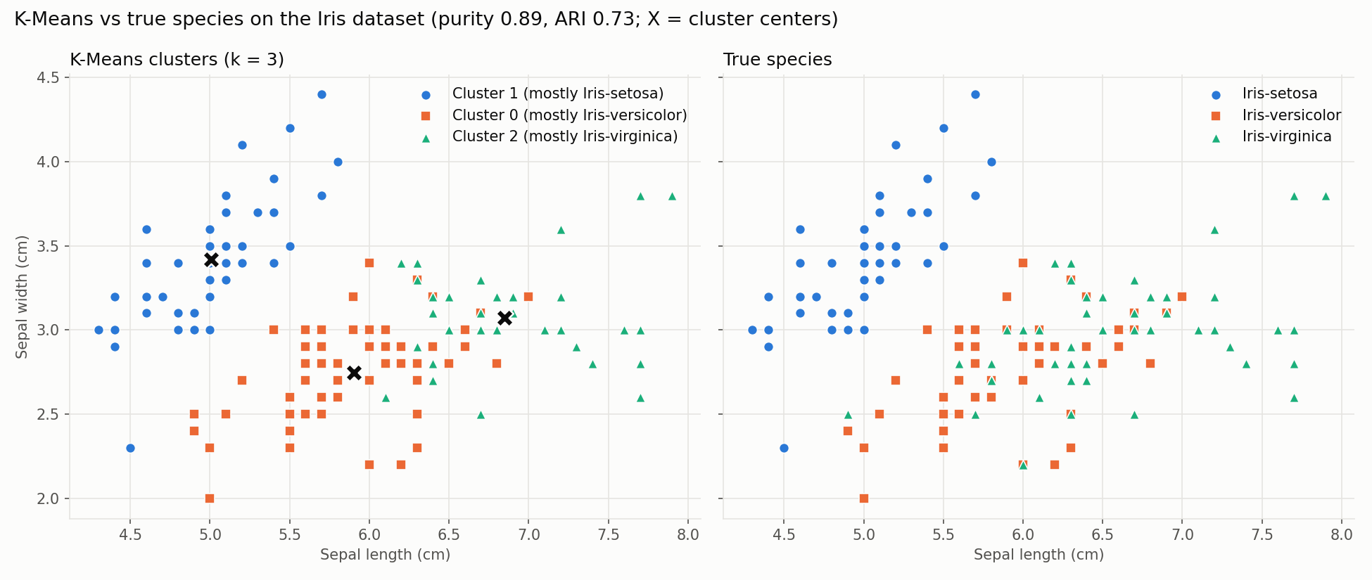
In the plots each cluster is paired one-to-one with the species it overlaps most (Hungarian algorithm, scipy.optimize.linear_sum_assignment) and given that species’ color and marker, which makes the left and right panels directly comparable despite the arbitrary cluster numbers.

Code

from sklearn.cluster import KMeans
from sklearn.metrics import adjusted_rand_score
import pandas as pd
 
kmeans = KMeans(n_clusters=3, n_init=10, random_state=0)
cluster_labels = kmeans.fit_predict(X)           # labels are NOT used for fitting
 
contingency = pd.crosstab(cluster_labels, y)     # clusters vs true species
purity = contingency.max(axis=1).sum() / contingency.values.sum()
ari = adjusted_rand_score(y, cluster_labels)

Related

• Supervised counterpart on the same data: Decision Trees
• Evaluation: Clustering Evaluation Metrics
• Source: scikit-learn clustering guide