Scale Space and Difference of Gaussians

An object can appear at any size, so a detector that looks at one fixed window size misses most of them. Scale space solves this by looking at the image at all scales at once: a feature is reported together with the scale at which it is strongest.

Scale Space

A scale space is the family of progressively blurred copies of the image:

$L(x,y,\sigma )=G(x,y,\sigma )\ast I(x,y)$

where $G$ is a Gaussian of width $\sigma$ (Gaussian Filtering and Convolution). Small $\sigma$ keeps fine detail, large $\sigma$ keeps only coarse structure, and $\sigma$ plays the role of scale. The Gaussian is the standard choice because blurring with it does not create new structure (no new extrema appear as $\sigma$ grows).

Blob Detection With the Laplacian

A blob is a bright or dark region of roughly constant intensity. The Laplacian of Gaussian responds strongly to a blob when its width matches the blob’s size. For this to be comparable across scales the response must be scale-normalized:

${\text{LoG}}_{norm}(x,y,\sigma )={\sigma }^2{\nabla }^{2}G\ast I$

A disc of radius $r$ gives its strongest response at $\sigma =r/\sqrt{2}$, so a blob found at scale $\sigma$ has radius about $\sqrt{2}\sigma$. Maxima and minima of ${\sigma }^2{\nabla }^{2}G$ were found to be more stable image features than the gradient, the Hessian or the Harris function.

Difference of Gaussians

The difference of Gaussians (DoG) approximates the normalized Laplacian cheaply. Subtract two blurred copies whose scales differ by a factor $k$:

$D(x,y,\sigma )=L(x,y,k\sigma )-L(x,y,\sigma )\approx (k-1){\sigma }^2{\nabla }^{2}G\ast I$

The factor $(k-1)$ is constant, so extrema are in the same places as for the true normalized Laplacian. The blurred images are needed anyway, so the DoG costs just one subtraction per level.

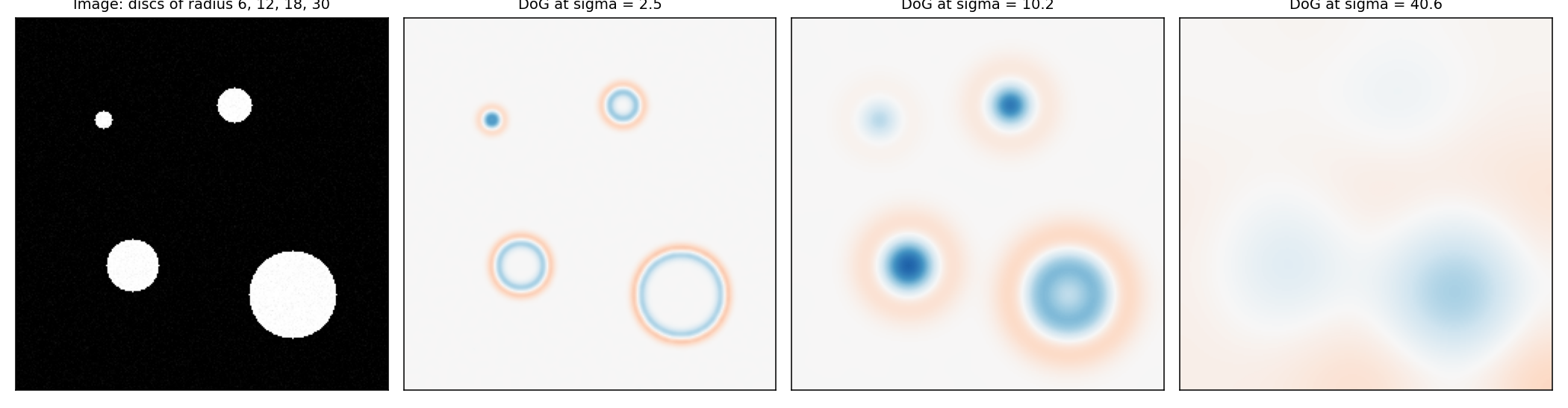
A test image with four discs and its DoG at three scales. Red and blue mark opposite signs. Each disc lights up most strongly at the level matching its size.

Octaves and Levels

Scale space is built in octaves, each covering a doubling of $\sigma$:

• Split each octave into $s$ steps, so consecutive levels differ by $k=2^{1/s}$.
• Produce $s+3$ blurred images per octave. That gives $s+2$ DoG images, so extrema can be checked at $s$ scales per octave using both the level above and the level below.
• After an octave, take the blurred image that has twice the starting $\sigma$ and keep every second pixel in each direction. This starts the next octave at half resolution without extra blurring, which is the same idea as an Image Pyramids level and avoids aliasing (Aliasing and Downsampling).

Extrema are found by comparing each DoG sample with its 26 neighbours (3 x 3 in its own level and the two adjacent levels). SIFT uses $s=3$ and a base blur of $\sigma =1.6$.

Worked Example

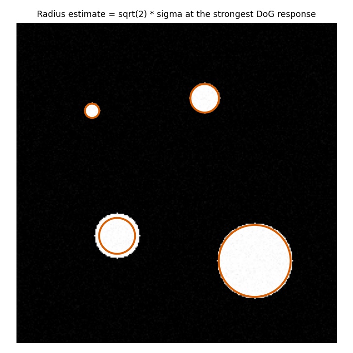
Circle radius is $\sqrt{2}\sigma$ at the level of the strongest DoG response at each disc centre. For discs of true radius 6, 12, 18 and 30, the estimates are 5.7, 11.4, 14.4 and 28.7. Scale is sampled in steps of about 26% ($k\approx 1.26$), which limits how close the estimate can be. The 18 estimate lands one step low.

Why It Matters

• Scale invariance: the same structure at two sizes peaks at two different $\sigma$, so detections in zoomed images match up after dividing out the scale (SIFT).
• Scale-adapted corners: Harris is not scale invariant (Harris Corner Detector), and scale-space versions search for extrema over $\sigma$ as well as position.
• Edges and noise: blurring suppresses noise before differentiation, as in Image Gradients and the Sobel Operator.

Sources: Lowe, Distinctive Image Features from Scale-Invariant Keypoints, IJCV 2004, for the DoG approximation, $s+3$ levels, octave resampling and 26-neighbour search. The radius relation $r=\sqrt{2}\sigma$ for discs and the no-new-extrema property are standard scale-space results from my own knowledge, and the radius numbers come from my own run on a synthetic test image.

---

Related: Computer Vision MOC, SIFT, Image Pyramids, Gaussian Filtering and Convolution