Vector Operations:
- Addition
- Scalar multiplication
Linear Combinations (c, d, e $\in \mathbb{R}$):
- cu + dv
- cu + dv + ew
Properties of Dot Product:
- Distributive: $u^T(v + w) = u^Tv+u^Tw$
- Non-Associative: $u^T(v^Tw) \ne (u^Tv)^Tw$
- Commutative: $u^Tv = v^Tu$
Cosine Formula for Dot Product: $v^Tw = |v| . |w| . cos(θ)$ (note: cos(θ) = 0 when θ = 90°)
Length of a vector: $\left| \mathbf{v} \right| = \sqrt{v_1^2 + v_2^2 + v_3^2 + …}$
Matrix operations:
- Addition (both matrices should have the same dimensions)
- Scalar multiplication
- Transpose: mapping A ∈ $\mathbb{R}^{n \times m}$ to B ∈ $\mathbb{R}^{m \times n}$ with $a_{ij} = b_{ji}$
- Trace: sum of all the elements along the diagonal
- Matrix multiplication (reminder: A∈$\mathbb{R}^{n \times m}$ and B∈$\mathbb{R}^{m \times k}$ then C=AB∈$\mathbb{R}^{n \times k}$)
Multiplication Properties:
- Distributivity: $(A +B)C = AC+BC$ and $A(C+D) =AC+AD$
- Associativity: $(AB)C = A(BC)$
- Non-commutative: $AB \ne BA$ (because of dimensions)
- Multiplication with the identity matrix results in the matrix itself
Properties of Transpose:
- $(A+B)^T =A^T +B^T$ and $(A - B)^T =A^T - B^T$
- $(AB)^T =B^TA^T$
Symmetric Matrices:
- $A^TB = B^TA$ if $A^TB$ is symmetric
Systems of Linear Equations Recap:
- $Ax = b$
- Gaussian Elimination
- Row Echelon/Reduced Row Echelon Form
A matrix is in row echelon form if
- all rows having only zero entries are at the bottom
- The pivot (the leftmost non-zero entry) of every non-zero row, called the pivot, is to the right of the leading entry of every row above
A matrix is in reduced row echelon form if:
- it is in row echelon form
- the leading entry in each nonzero row is 1 (called a leading one)
- each column containing a leading 1 has zeros in all its other entries (or in other words, above the pivot if condition one is achieved)
Properties of Determinants:
- Matrix must be square
- The determinant of the identity matrix is 1.
- The exchange of two rows multiplies the determinant by −1.
- Multiplying a row or a column by a number multiplies the determinant by this number.
- Adding a multiple of one row to another row does not change the determinant.
- If two rows of matrix A are equal, then $det(A) = 0$.
- A matrix with a row of zeros has $det(A) = 0$.
- If A is triangular then $det(A)$ is the product of diagonal entries.
- $det(AB) = det(A).det(B)$
- $det(A^T) = det(A)$
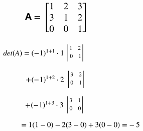
Laplace Expansion Example:
Invertibility:
- Matrix must be square
- If A is singular, then $det(A) = 0$. If A is invertible, then $det(A) \ne 0$.
- Can calculate the inverse using Gaussian Elimination
- $[A \vert I]$ -> $[I \vert A^-1]$
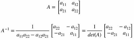
- Inverse for a 2x2:
Vector Spaces and Subspaces
A subspace is defined as a set of all vectors that can be created by taking linear combinations of some vectors or a set of vectors.
Formally, a subspace is the set of all vectors that satisfy the following conditions:
- Must be closed under addition and multiplication
- Must contain the zero vector
Note
A vector space needs to contain all linear combinations of its vectors.
Example 1: Possible subspaces
| Dimension | Subspaces in $R^2$: | Subspaces in $R^3$: |
|---|---|---|
| 0 | The zero vector | The zero vector |
| 1 | Lines that pass through the origin | Lines that pass through the origin |
| 2 | All of $R^2$ | Planes that pass through the origin |
| 3 | - | All of $R^3$ |
Dimension of a subspace
The dimension of a subspace is always ≤ the dimension of the space it lives in.
Example 2: What does NOT qualify as a subspace? Think about a line that doesn’t pass through the origin - say, all points where $y = x + 1$. If we pick a vector on that line, like (0, 1), and we multiply it by the scalar 0, we get (0, 0) - which is NOT on the line $y = x + 1$. So that line isn’t closed under scalar multiplication, and therefore can’t be a subspace.
The distinction:
- While $y = x + 1$ is contained in ℝ² (every point on the line is in ℝ² - (0,1), (1,2), (2,3) etc.)
- It is NOT a subspace of ℝ² (doesn’t contain zero vector, not closed under operations)
- Therefore, it does not qualify as (does not form) a subspace.
The four fundamental subspaces of $A_{mxn}$
| Name | Dim | Note |
|---|---|---|
| Column Space | C(A)∈$R^m$ | Pivot columns of the original matrix |
| Null Space | N(A)∈$R^n$ | - Solve $Ax=0$, set free column variables to 1 respectively - # of free columns = dimension of null space |
| Row Space | C($A^T$)∈$R^n$ | Pivot rows |
| Left Null Space | N($A^T$)∈$R^m$ | Solve for y where $y^T.A=0$ |
Dimensions
For matrix A with dimensions $m$x$n$:
- $dim(C(A)) + dim(N(A)) = n$ (# of columns)
- $dim(C(A^T)) + dim(N(A^T)) = m$ (# of rows)
Orthogonal Subspaces
- $N(A) \bot C(A^T)$
- $N(A^T) \bot C(A)$
If the null space is {(0,0,0)} then (only consists of the zero vector),
- Dimension of null space = 0
- Number of free columns = 0
- All columns are pivot columns
Null space of A
If vector $\vec{v}$ is in the null space of matrix A, then A$\vec{v}=0$.
Complete Solution System of Linear Equations $x_{particular}$ : Set all free variables to 0, then solve $Ax=b$ (or $Rx=b$ where R is the echelon/reduced echelon form)
$x_{null space}$ : Set free columns to 1 and solve $Rx=0$. If there are more than one, set them respectively. For example, if there are two free variables (let’s say $x_2$ and $x_3$) first set $x_2 = 1$, $x_3 = 0$ and solve for $Rx=0$. Then set $x_2 = 0$, $x_3 = 1$ and solve for $Rx=0$. Two free variables mean there will be two special solutions.
A system’s solution set has three possibilities:
- unique solution
- infinite solutions
- no solution
If $det(A) = 0$ the system has either,
- no solution OR
- infinitely many solutions
Rank
- Matrix rank = # of pivots
- In a square matrix, if the rank < # of columns that means there are linearly dependent rows, thus the matrix is not invertible ($det(A) = 0$)
- The rank of A = # of independent rows = # of independent columns (very important)
Basis
Tip for Finding the Span
If we want to find that in the span of , we can just look at the rank of If the rank is smaller than the number of columns, can be expressed as a linear combination of the other vectors. In this case, the rank is <3 so yes, $\vec{v}$ is in the span of S.
Why use different bases?
- Simplification: Some problems become way easier in a different basis
- Example: In physics, choosing a basis aligned with forces makes calculations simpler
- Natural coordinates: Sometimes a problem has a natural coordinate system
- Example: If you’re studying oscillations, sine and cosine functions form a natural basis
- Revealing structure: Different bases can reveal hidden patterns in data
- Example: Principal Component Analysis (PCA) in data science finds a basis that shows the most important directions in your data
Changing Basis
Solve for $\vec{w}$ where the basis A, B and $\vec{v}$ is known: $A.\vec{v} = B.\vec{w}$ You get $\vec{w}$ represented in basis B.
Orthogonality
- Two vectors are orthogonal if their dot product is 0.
- Two subspaces $V$ and $W$ of a vector space are orthogonal if every vector in $V$ is perpendicular to every vector in $W$.
- The null space $N(A)$ and the row space $C(A^T)$ are orthogonal subspaces of $R^n$.
- The left null space $N(A^T)$ and the column space $C(A)$ are orthogonal subspaces of $R^m$.
Projections
The projection of $b$ onto a subspace $S$ is the closest vector $p$ in $S$. A projection matrix $P$ is a symmetric matrix with $P^2=P$. The projection of is $b$ is given by $Pb$.
Projection onto a line
- x is a scalar.
Projection onto a Subspace
- x is a scalar.
Theorem: If $A$ has linearly independent columns then $A^TA$ is invertible.
Least Squares Approximation
- Solve $A^TAx = A^Tb$ where
and $y=c+mx$
Orthonormal Vectors
Vectors $q_1, …, q_n$ are orthonormal if $q_i^Tq_j=$
- 0 when $i\neq j$
- 1 when $i=j$
Assume A has orthonormal column, then we can find the projection matrix using
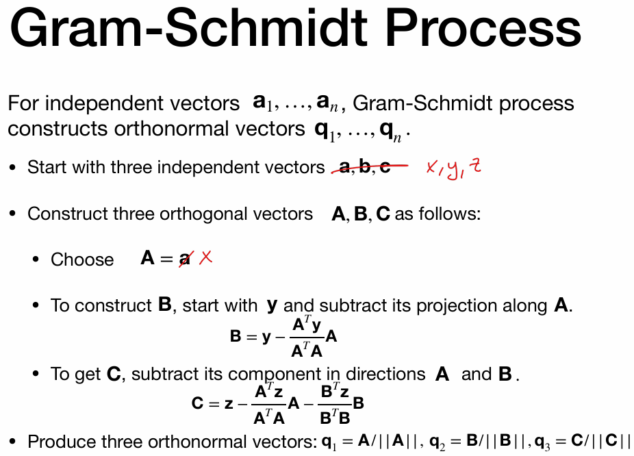
Gram-Schmidt Process
Eigenvectors & Eigenvalues
If, then $v$ is an eigenvector of A with eigenvalue $\lambda$. In other words, $Av$ lies in the same one-dimensional subspace as $\lambda v$.
Finding eigenvectors:
$(A - \lambda I)$ should have a non-trivial null space. Which means it is singular and $det(A - \lambda I)=0$.
Diagonalization
$AV = VΛ$ where $Λ$ is the diagonal eigenvalue matrix and $V$ is the eigenvector matrix.
Spectral Theorem
For a symmetric matrix $S$, the following diagonalization can be written:
where $Q$ is the orthonormal eigenvector matrix. i.e. eigenvectors of a real symmetric matrix are always perpendicular.
Singular Value Decomposition
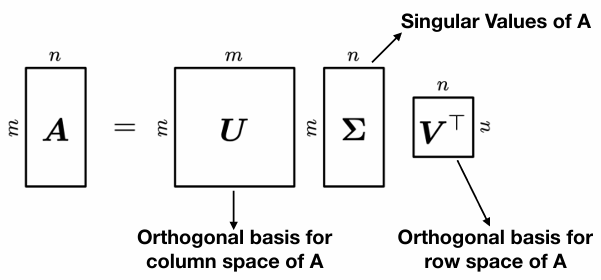
Tip: SVD can be used for dimensionality reduction or compression.
or,
Once you find $V$ and $\varepsilon$, find $U$ by calculating $Av_i = \sigma_i u_i$ where $v$ and $u$ are eigenvectors of $V$ and $U$. $\sigma_i$ is the square root of eigenvalues obtained from $\varepsilon^2$.
Important note: $V$ and $U$ should have unit eigenvectors. Also, sort eigenvectors from in descending order of corresponding eigenvalues.